[ad_1]
Introduction
Many deep studying developments will be attributed to will increase in (1) information dimension and (2) computational energy. Coaching deep studying fashions with bigger datasets will be extraordinarily useful for mannequin coaching. Not solely do they assist stabilize mannequin efficiency throughout coaching, however analysis exhibits that for average to large-scale fashions and datasets, mannequin efficiency converges as a power-law with coaching information dimension, that means we are able to predict enhancements to mannequin accuracy because the dataset grows.
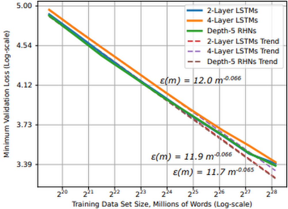
Determine 1: Studying curve and dataset dimension for phrase language fashions (supply)
In follow this implies as we glance to enhance mannequin efficiency with bigger datasets, (1) we’d like entry to hardware accelerators, reminiscent of GPUs or TPUs, and (2) we have to architect a system that effectively shops and delivers this information to the accelerators. There are a couple of the reason why we could select to stream information from distant storage to our accelerator gadgets:
- Information dimension: information will be too massive to suit on a single machine, requiring distant storage and environment friendly community entry
- Streamlined workflows: transferring information to disk will be time consuming and useful resource intensive, we wish to make fewer copies of the information
- Collaboration: disaggregating information from accelerator gadgets means we are able to extra effectively share accelerator nodes throughout workloads and groups
Streaming coaching information from distant storage to accelerators can alleviate these points, however it introduces a number of latest challenges:
- Community overhead: Many datasets encompass thousands and thousands of particular person information, randomly accessing these information can introduce community bottlenecks. We want sequential entry patterns
- Throughput: Fashionable accelerators are quick; the problem is feeding them quick sufficient to maintain them totally utilized. We want parallel I/O and pipelined entry to information
- Randomness vs Sequential: The optimization algorithms in deep studying jobs profit from randomness, however random file entry introduces community bottlenecks. Sequential entry alleviates community bottlenecks, however can cut back the randomness wanted for coaching optimization. We have to stability these
How can we architect a system that addresses these challenges at scale?
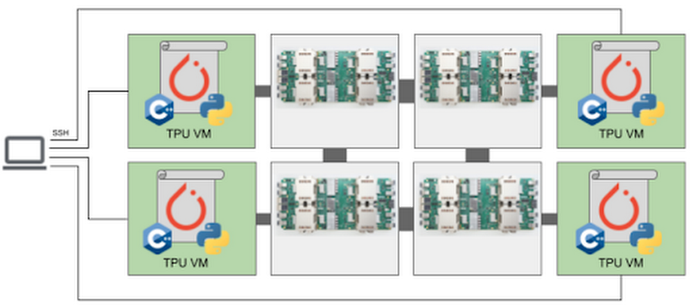
Determine 2: Scaling to bigger datasets, extra gadgets
On this publish, we’ll cowl:
- The challenges related to scaling deep studying jobs to distributed coaching settings
- Utilizing the brand new Cloud TPU VM interface
- Methods to stream coaching information from Google Cloud Storage (GCS) to PyTorch / XLA fashions operating on Cloud TPU Pod slices
You will discover accompanying code for this text on this GitHub repository.
Mannequin and dataset
On this article, we’ll prepare a PyTorch / XLA ResNet-50 mannequin on a v3-32 TPU Pod slice the place coaching information is saved in GCS and streamed to the TPU VMs at coaching time. ResNet-50 is a 50-layer convolutional neural community generally used for laptop imaginative and prescient duties and machine studying efficiency benchmarking. To display an end-to-end instance, we’ll use the CIFAR-10 dataset. The unique dataset consists of 60,000 32×32 shade photographs divided into 10 lessons, every class containing 6,000 photographs. We’ve upsampled this dataset, making a coaching and take a look at set of 1,280,000 and 50,000 photographs, respectively. CIFAR is used as a result of it’s publicly accessible and well-known; nevertheless, within the GitHub repository, we offer steering for adapting this resolution to your workloads, in addition to bigger datasets reminiscent of ImageNet.
Cloud TPU
TPUs, or Tensor Processing Items, are ML ASICs particularly designed for large-scale mannequin coaching. As they excel at any job the place massive matrix multiplications dominate, they will speed up deep studying jobs and cut back the overall price of coaching. In the event you’re new to TPUs, verify this text to grasp how they work.
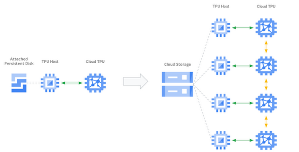
The v3-32 TPU used on this instance consists of 32 TPU v3 cores and 256 GiB of whole TPU reminiscence. This TPU Pod slice consists of four TPU Boards (a Board has eight TPU cores). Every TPU Board is related to a high-performance CPU-based host machine for issues like loading and preprocessing information to feed to the TPUs.
We’ll entry the TPU via the brand new Cloud TPU VMs. After we use Cloud TPU VMs, a VM is created for every TPU board within the configuration. Every VM consists of 48 vCPUs and 340 GB of reminiscence, and comes preinstalled with the newest PyTorch / XLA picture. As a result of there is no such thing as a consumer VM, we ssh straight into the TPU host to run our mannequin and code. This root entry eliminates the necessity for a community, VPC, or firewall between our code and the TPU VM, which may considerably enhance the efficiency of our enter pipeline. For extra particulars on Cloud TPU VMs, see the System Structure.
PyTorch / XLA
PyTorch / XLA is a Python library that makes use of the XLA (Accelerated Linear Algebra) deep studying compiler to attach PyTorch and Cloud TPUs. Try the GitHub repository for tutorials, finest practices, Docker Photos, and code for widespread fashions (e.g., ResNet-50 and AlexNet).
Information parallel distributed coaching
Distributed coaching usually refers to coaching workloads which use a number of accelerator gadgets (e.g. GPU or TPU). In our instance, we’re executing a knowledge parallel distributed coaching job with stochastic gradient descent. In information parallel coaching, our mannequin suits on a single TPU system and we replicate the mannequin throughout every system in our distributed configuration. After we add extra gadgets, our objective is to cut back general coaching time by distributing non-overlapping partitions of the coaching batch to every system for parallel processing. As a result of our mannequin is replicated throughout gadgets, the fashions on every system want to speak to synchronize their weights after every coaching step. In distributed information parallel jobs, this system communication is usually finished both asynchronously or synchronously.
Cloud TPUs execute synchronous system communication over the devoted high-speed community connecting the chips. In our mannequin code, we use PyTorch / XLA’s optimizer_step(optimizer) to calculate the gradients and provoke this synchronous replace.
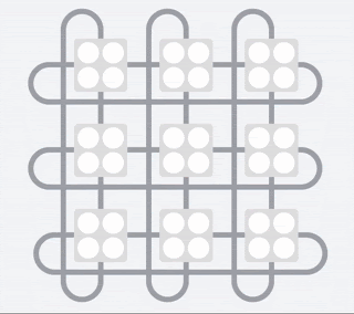
Determine four: Synchronous all-reduce on Cloud TPU interconnect
After the native gradients are computed, the xm.optimizer_step() perform synchronizes the native gradients between cores by making use of an AllReduce(SUM) operation, after which calls the PyTorch optimizer_step(optimizer), which updates the native weights with the synchronized gradients. On the TPU, the XLA compiler generates AllReduce operations over the devoted community connecting the chips. In the end, the globally averaged gradients are written to every mannequin duplicate’s parameter weights, guaranteeing the replicas begin from the identical state in each coaching iteration. We are able to see the decision to this perform within the coaching loop:
Enter pipeline efficiency
As beforehand talked about, the problem with TPUs is feeding them the coaching information quick sufficient to maintain them busy. This downside exists once we retailer coaching information on an area disk and turns into much more clear once we stream information from distant storage. Let’s first evaluation a typical machine studying coaching loop.
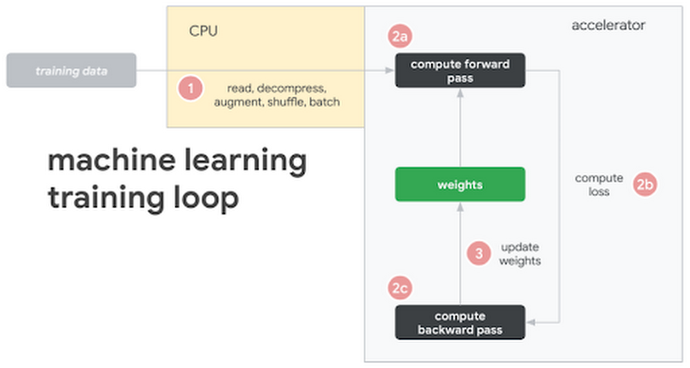
Determine 5: Frequent machine studying coaching loop and hardware configuration
On this illustration, we see the next steps:
- Coaching information is both saved on native disk or distant storage
- The CPU (1) requests and reads the information, augments it with varied transformations, batches it, and feeds it to the mannequin
- As soon as the mannequin has the remodeled, batched coaching information, (2) the accelerator takes over
- The accelerator (2a) computes the ahead move, (2b) loss, and (2c) backwards move
- After computing the gradients, (three) the parameter weights are up to date (the training!)
- And we repeat the cycle over once more
Whereas this sample will be tailored in a number of methods (e.g., some transformations may very well be computed on the accelerator), the prevailing theme is that a perfect structure seeks to maximise utilization of the costliest element, the accelerator. And due to this, we see most efficiency bottlenecks occurring within the enter pipeline pushed by the CPU. To assist with this, we’re going to use the WebDataset library. WebDataset is a PyTorch dataset implementation designed to enhance streaming information entry for deep studying workloads, particularly in distant storage settings. Let’s see the way it helps.
WebDataset format
WebDatasets are simply POSIX tar archive information, and they are often created with the well-known tar command. They do not require any information conversion; the information format is similar within the tar file as it’s on disk. For instance, our coaching photographs are nonetheless in PPM, PNG, or JPEG format when they’re saved and transferred to the enter pipeline. The tar format gives efficiency enhancements for each small and enormous datasets, in addition to information saved on both native disk or distant storage, reminiscent of GCS. Let’s define three key pipeline efficiency enhancements we are able to obtain with WebDataset.
(1) Sequential I/O
GCS is able to sustaining excessive throughput, however there’s some community overhead when initiating a connection. If we’re accessing thousands and thousands of particular person picture information, this isn’t excellent. Alternatively, we are able to obtain sequential I/O by requesting a tar file containing our particular person picture information. As soon as we request the tar file, we get sequential reads of the person information inside that tar file, which permits for sooner object I/O over the community. This reduces the variety of community connections to ascertain with GCS, and thus reduces potential community bottlenecks.
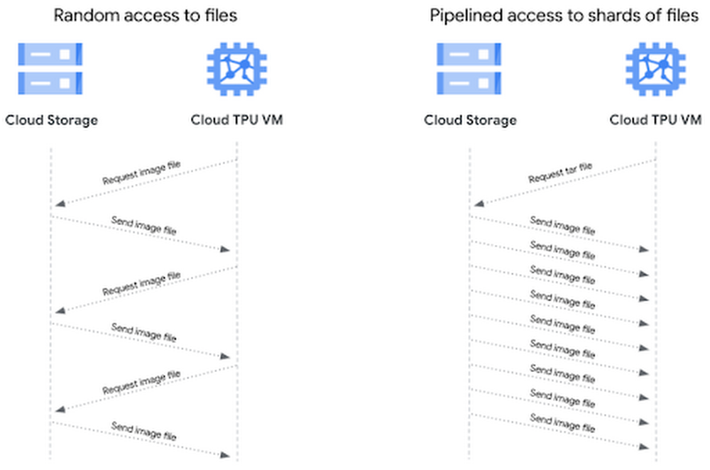
Determine 6: Evaluating random and pipelined entry to information information
(2) Pipelined information entry
With file-based I/O we randomly entry picture information, which is sweet for coaching optimization, however for every picture file there’s a consumer request and storage server response. Our sequential storage achieves increased throughput as a result of with a single consumer request for a tar file, the information samples in that file stream sequentially to the consumer. This sample provides us pipelined entry to our particular person picture information, leading to increased throughput.
(three) Sharding
Storing TBs of knowledge in a single sequential file may very well be troublesome to work with and it prevents us from attaining parallel I/O. Sharding the dataset might help us in a number of methods:
- Mixture community I/O by opening shards in parallel
- Speed up information preprocessing by processing shards in parallel
- Randomly entry shards, however learn sequentially inside every shard
- Distribute shards effectively throughout employee nodes and gadgets
- Assure equal variety of coaching samples on every system
As a result of we are able to management the variety of shards and the variety of samples in these shards, we are able to distribute equal-sized shards and assure every system receives the identical variety of samples in every coaching epoch. Sharding the tar information helps us stability the tradeoff between random information entry and sequential reads. Random entry to the shards and in-memory shuffling fulfill sufficient randomness for the coaching optimization. The sequential reads from every shard cut back community overhead.
Distributing shards throughout gadgets and employees
As we’re basically making a PyTorch IterableDataset, we are able to use the PyTorch DataLoader to load information on the gadgets for every coaching epoch. Conventional PyTorch Datasets distribute information on the sample-level, however we’re going to distribute on the shard-level. We’ll create two capabilities to deal with this distribution logic and move them to the `splitter=` and `nodesplitter=` arguments once we create our dataset object. All these capabilities must do is take a listing of shards and return a subset of these shards. (To see how the next snippets match into the mannequin script, try test_train_mp_wds_cifar.py within the accompanying GitHub repository.)
We’ll break up shards throughout employees with:
We’ll break up shards throughout gadgets with:
With these two capabilities we’ll create a knowledge loader for each prepare and validation information. Right here is the prepare loader:
Right here is an evidence of a number of the variables utilized in these snippets:
xm.xrt_world_size()is the overall variety of gadgets, or TPU coresFLAGS.num_workersis the variety of subprocesses spawned per TPU core for loading and preprocessing information- The
epoch_sizespecifies the variety of coaching samples every system ought to count on for every epoch shardshuffle=Truemeans we’ll shuffle the shards, whereas.shuffle(10000)shuffles samples inline.batched(batch_size, partial=True)explicitly batches information within the Dataset bybatch_sizeand‘partial=True’handles partial batches, usually discovered within the final shard- Our loader is a typical PyTorch DataLoader. As a result of our WebDataset Dataset accounts for batching, shuffling, and partial batches, we don’t use these arguments in PyTorch’s DataLoader
Efficiency comparability
The desk in Determine 7 compares the efficiency between three completely different coaching configurations for a PyTorch / XLA ResNet-50 mannequin coaching on the ImageNet dataset. Configuration A gives baseline metrics and represents a mannequin studying from native storage, randomly accessing particular person picture information. Configuration B makes use of an identical setup as A, besides the coaching information is sharded into 640 POSIX tar information and the WebDataset library is used to pattern and distribute shards to the mannequin replicas on Cloud TPU gadgets. Configuration C makes use of the identical sampling and distribution logic as B, however sources coaching information from distant storage in GCS. The metrics signify a median of every configuration over 5 90-epoch coaching jobs.
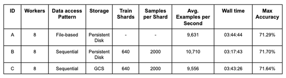
Determine 7: Coaching efficiency comparability
Evaluating configurations A and B, these outcomes present that merely utilizing a sharded, sequentially readable information format improves pipeline and mannequin throughput (common examples per second) by 11.2%. In addition they present that we are able to make the most of distant storage with out negatively impacting mannequin coaching efficiency. Evaluating configurations A and C, we have been in a position to preserve pipeline and mannequin throughput, coaching time, and mannequin accuracy.
To focus on the impacts of sequential and parallel I/O, we held many configuration settings fixed. There are nonetheless a number of areas to analyze and enhance. In a later publish we’ll present the best way to use the Cloud TPU profiler device to additional optimize PyTorch / XLA coaching jobs.
Finish-to-end instance
Let’s stroll via a full instance.
To comply with this instance, you should use this pocket book to create a sharded CIFAR dataset.
Earlier than you start
Within the Cloud Shell, run the next instructions to configure gcloud to make use of your GCP undertaking, set up elements wanted for the TPU VM preview, and allow the TPU API. For extra TPU 1VM setup particulars, see these directions.
Connecting to a Cloud TPU VM
The default community comes preconfigured to permit ssh entry to all VMs. In the event you don’t use the default community, or the default community settings have been edited, chances are you’ll must explicitly allow SSH entry by including a firewall rule:
At the moment within the TPU VM preview, we suggest disabling OS login to permit native scp (required for PyTorch / XLA Pods).
Making a TPU 1VM slice
We’ll create our TPU Pod slice in europe-west4-a as a result of this area helps each TPU VMs and v3-32 TPU Pod slices.
-
TPU_NAME: identify of the TPU node -
ZONE: location of the TPU node -
ACCELERATOR_TYPE: discover the record of supported accelerator sorts right here -
RUNTIME_VERSION: for PyTorch / XLA, use v2-alpha for single TPUs and TPU pods. This can be a secure model for our public preview launch.
PyTorch / XLA requires all TPU VMs to have the ability to entry the mannequin code and information. Utilizing gcloud, we’ll embody a metadata startup-script which installs the mandatory packages and code on every TPU VM.
This command will create a v3-32 TPU Pod slice and four VMs, one devoted to every TPU board.
To ssh right into a TPU VM, we’ll use the gcloud ssh command under. By default, this command will hook up with the primary TPU VM employee (denoted with w-Zero). To ssh into another VM related to the TPU Pod, append `--worker $` within the command, the place the WORKER_NUMBER is Zero-based. See right here for extra particulars on managing TPU VMs.
As soon as within the VM, run the next command to generate the ssh-keys to ssh between VM employees on a pod:
PyTorch coaching
Test to ensure the metadata startup script has cloned all of the repositories. After operating the next command, we should always see the torchxla_tpu listing.
To coach the mannequin, let’s first arrange some setting variables:
BUCKET: identify of GCS bucket storing our sharded dataset. We can even retailer coaching logs and mannequin checkpoints right here (see tips on GCS object names and folders)_SHARDS: prepare/val shards, utilizing brace notation to enumerate the shardsWDS__DIR: makes use of pipe to run agsutilcommand for downloading the prepare/val shardsLOGDIR:location in GCS bucket for storing coaching logs
Optionally, we are able to move setting variables for storing mannequin checkpoints and loading from a earlier checkpoint file:
After we select to save lots of mannequin checkpoints, a checkpoint file will likely be saved on the finish of every epoch if the validation accuracy improves. Every time a checkpoint is created, the PyTorch / XLA xm.save() utility API will save the file domestically, overwriting any earlier file if it exists. Then, utilizing the Cloud Storage Python SDK, we’ll add the file to the desired $LOGDIR, overwriting any earlier file if it exists. Our instance saves a dictionary of related data like this:
Right here is the perform that makes use of the Cloud Storage SDK to add every mannequin checkpoint to GCS:
If we wish to resume coaching from a earlier checkpoint, we use the LOAD_CHKPT_FILE variable to specify the GCS object to obtain and the LOAD_CHKPT_DIR variable to specify the native listing to position this file. As soon as the mannequin is initialized, we deserialize the dictionary with torch.load(), load the mannequin’s parameter dictionary with load_state_dict(), and transfer the mannequin to the gadgets with .to(system).
Right here is the perform that makes use of the Cloud Storage SDK to obtain the checkpoint and reserve it to an area listing:
We are able to use different data from our dictionary to configure the coaching job, reminiscent of updating the very best validation accuracy and epoch:
If we don’t wish to save or load these information, we are able to omit them from the command line arguments. Particulars on saving and loading PyTorch / XLA checkpoint information will be discovered right here.
Now we’re prepared to coach.
-
--restart-tpuvm-pod-serverrestarts the XRT_SERVER (XLA Runtime) and is helpful when operating consecutive TPU jobs (particularly if that server was left in a nasty state). For the reason that XRT_SERVER is persistent for the pod setup, setting variables received’t be picked up till the server is restarted. -
test_train_mp_wds_cifar.pycarefully follows the PyTorch / XLA distributed, multiprocessing script, however is tailored to incorporate help for WebDataset and CIFAR -
TPUs have hardware help for Mind Floating Level Format, which can be utilized by setting
XLA_USEBF16=1
Throughout coaching, output for every step seems to be like this:
10.164.Zero.25refers back to the IP tackle for this VM employee[0]refers to VM employee Zero. Recall, there are four VM employees in our instanceCoaching System=xla:Zero/2refers back to the TPU core 2. In our instance there are 32 TPU cores, so it is best to see as much asxla:Zero/31(since they’re Zero-based)Fee=1079.01refers back to the exponential transferring common of examples per second for this TPU coreGlobalRate=1420.67refers back to the common variety of examples per second for this core thus far throughout this epoch
On the finish of every epoch’s prepare loop, you will notice output like this:
Duplicate Practice Samplestells us what number of coaching samples this duplicate processedDecreased GlobalRateis the common GlobalRate throughout all replicas for this epoch
As soon as coaching is full, you will notice the next output:
The logs for every VM employee are produced asynchronously, so it may be troublesome to learn them sequentially. To view the logs sequentially for any TPU VM employee, we are able to execute the next command, the place the IP_ADDRESS is the tackle to the left of our [0].
We are able to convert these to a.txt file and retailer them in a GCS bucket like this:
Cleansing up
We are able to clear up our TPU VM sources in a single easy command.
First, disconnect from the TPU VM, when you have not already finished so:
Within the Cloud Shell, use the next command to delete the TPU VM sources:
In the event you want to delete the GCS bucket and its contents, run the next command within the Cloud Shell terminal:
What’s subsequent?
On this article we explored the challenges of utilizing distant storage in distributed deep studying coaching jobs. We mentioned the benefits of utilizing sharded, sequentially readable information codecs to unravel the challenges with distant storage entry and the way the WebDataset library makes this simpler with PyTorch. We then walked via an instance demonstrating the best way to stream coaching information from GCS to TPU VMs and prepare a PyTorch / XLA mannequin on Cloud TPU Pod slices.
References
- Cloud TPUs
- Cloud TPU 1VM structure
- PyTorch XLA GitHub repository
- WebDataset GitHub repository
- GitHub repository for this code
Within the subsequent installment of this sequence, we’ll revisit this instance and work with Cloud TPU Instruments to additional optimize our coaching job. We’ll display how variables reminiscent of shard dimension, shard rely, batch dimension, and variety of employees impression the enter pipeline, useful resource utilization, examples per second, accuracy, loss, and general mannequin convergence.
Have a query or wish to chat? Discover the authors right here – Jordan and Shane.
Particular because of Karl Weinmeister, Rajesh Thallam, and Vaibhav Singh for his or her contributions to this publish, in addition to Daniel Sohn, Zach Cain, and the remainder of the PyTorch / XLA group for his or her efforts to reinforce the PyTorch expertise on Cloud TPUs.
[ad_2]
Source link