[ad_1]

|
With Amazon Redshift, you should use SQL to question and mix exabytes of structured and semi-structured information throughout your information warehouse, operational databases, and information lake. Now that AQUA (Superior Question Accelerator) is usually obtainable, you’ll be able to enhance the efficiency of your queries by as much as 10 occasions with no extra prices and no code modifications. In actual fact, Amazon Redshift offers as much as thrice higher value/efficiency than different cloud information warehouses.
However what if you wish to go a step additional and course of this information to coach machine studying (ML) fashions and use these fashions to generate insights from information in your warehouse? For instance, to implement use instances comparable to forecasting income, predicting buyer churn, and detecting anomalies? Previously, you would wish to export the coaching information from Amazon Redshift to an Amazon Easy Storage Service (Amazon S3) bucket, after which configure and begin a machine studying coaching course of (for instance, utilizing Amazon SageMaker). This course of required many alternative expertise and often multiple particular person to finish. Can we make it simpler?
At this time, Amazon Redshift ML is typically obtainable that can assist you create, prepare, and deploy machine studying fashions immediately out of your Amazon Redshift cluster. To create a machine studying mannequin, you employ a easy SQL question to specify the info you need to use to coach your mannequin, and the output worth you need to predict. For instance, to create a mannequin that predicts the success price on your advertising actions, you outline your inputs by choosing the columns (in a number of tables) that embody buyer profiles and outcomes from earlier advertising campaigns, and the output column you need to predict. On this instance, the output column could possibly be one which reveals whether or not a buyer has proven curiosity in a marketing campaign.
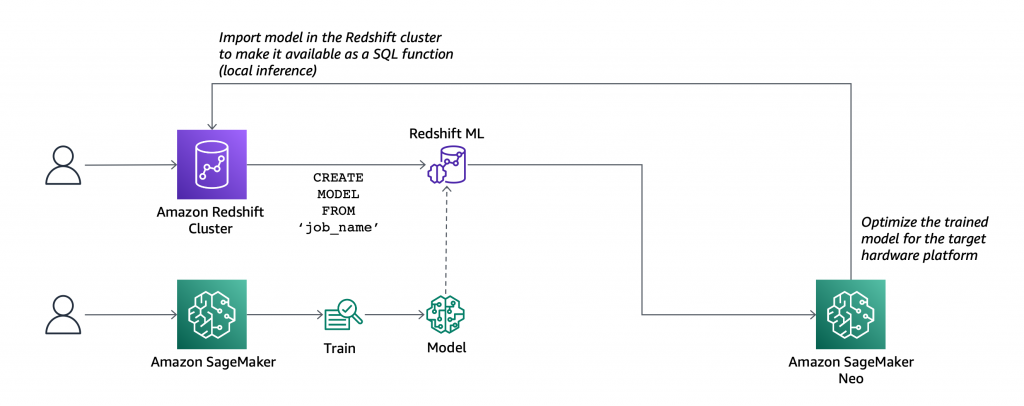
After you run the SQL command to create the mannequin, Redshift ML securely exports the desired information from Amazon Redshift to your S3 bucket and calls Amazon SageMaker Autopilot to organize the info (pre-processing and have engineering), choose the suitable pre-built algorithm, and apply the algorithm for mannequin coaching. You’ll be able to optionally specify the algorithm to make use of, for instance XGBoost.

Redshift ML handles the entire interactions between Amazon Redshift, S3, and SageMaker, together with all of the steps concerned in coaching and compilation. When the mannequin has been skilled, Redshift ML makes use of Amazon SageMaker Neo to optimize the mannequin for deployment and makes it obtainable as a SQL operate. You should utilize the SQL operate to use the machine studying mannequin to your information in queries, reviews, and dashboards.
Redshift ML now consists of many new options that weren’t obtainable throughout the preview, together with Amazon Digital Personal Cloud (VPC) help. For instance:
- You may as well create SQL features that use present SageMaker endpoints to make predictions (distant inference). On this case, Redshift ML is batching calls to the endpoint to hurry up processing.

Earlier than wanting into learn how to use these new capabilities in observe, let’s see the distinction between Redshift ML and comparable options in AWS databases and analytics companies.
Constructing a Machine Studying Mannequin with Redshift ML
Let’s construct a mannequin that predicts if clients will settle for or decline a advertising provide.
To handle the interactions with S3 and SageMaker, Redshift ML wants permissions to entry these assets. I create an AWS Identification and Entry Administration (IAM) position as described within the documentation. I exploit RedshiftML for the position title. Be aware that the belief coverage of the position permits each Amazon Redshift and SageMaker to imagine the position to work together with different AWS companies.
From the Amazon Redshift console, I create a cluster. Within the cluster permissions, I affiliate the RedshiftML IAM position. When the cluster is accessible, I load the identical dataset used on this tremendous fascinating weblog publish that my colleague Julien wrote when SageMaker Autopilot was introduced.
The file I’m utilizing (bank-additional-full.csv) is in CSV format. Every line describes a direct advertising exercise with a buyer. The final column (y) describes the end result of the exercise (if the shopper subscribed to a service that was marketed to them).
Listed here are the primary few traces of the file. The primary line incorporates the headers.
I retailer the file in one in all my S3 buckets. The S3 bucket is used to unload information and retailer SageMaker coaching artifacts.
Then, utilizing the Amazon Redshift question editor within the console, I create a desk to load the info.
CREATE TABLE direct_marketing (
	age DECIMAL NOT NULL,
	job VARCHAR NOT NULL,
	marital VARCHAR NOT NULL,
	schooling VARCHAR NOT NULL,
	credit_default VARCHAR NOT NULL,
	housing VARCHAR NOT NULL,
	mortgage VARCHAR NOT NULL,
	contact VARCHAR NOT NULL,
	month VARCHAR NOT NULL,
	day_of_week VARCHAR NOT NULL,
	period DECIMAL NOT NULL,
	marketing campaign DECIMAL NOT NULL,
	pdays DECIMAL NOT NULL,
	earlier DECIMAL NOT NULL,
	poutcome VARCHAR NOT NULL,
	emp_var_rate DECIMAL NOT NULL,
	cons_price_idx DECIMAL NOT NULL,
	cons_conf_idx DECIMAL NOT NULL,
	euribor3m DECIMAL NOT NULL,
	nr_employed DECIMAL NOT NULL,
	y BOOLEAN NOT NULL
);
I load the info into the desk utilizing the COPY command. I can use the identical IAM position I created earlier (RedshiftML) as a result of I’m utilizing the identical S3 bucket to import and export the info.
Now, I create the mannequin straight kind the SQL interface utilizing the brand new CREATE MODEL assertion:
CREATE MODEL direct_marketing
FROM direct_marketing
TARGET y
FUNCTION predict_direct_marketing
IAM_ROLE 'arn:aws:iam::123412341234:position/RedshiftML'
SETTINGS (
  S3_BUCKET 'my-bucket'
);
On this SQL command, I specify the parameters required to create the mannequin:
FROM– I choose all of the rows within thedirect_marketingdesk, however I can exchange the title of the desk with a nested question (see instance under).TARGET– That is the column that I need to predict (on this case,y).FUNCTION– The title of the SQL operate to make predictions.IAM_ROLE– The IAM position assumed by Amazon Redshift and SageMaker to create, prepare, and deploy the mannequin.S3_BUCKET– The S3 bucket the place the coaching information is quickly saved, and the place mannequin artifacts are saved for those who select to retain a duplicate of them.
Right here I’m utilizing a easy syntax for the CREATE MODEL assertion. For extra superior customers, different choices can be found, comparable to:
MODEL_TYPE– To make use of a selected mannequin sort for coaching, comparable to XGBoost or multilayer perceptron (MLP). If I don’t specify this parameter, SageMaker Autopilot selects the suitable mannequin class to make use of.PROBLEM_TYPE– To outline the kind of downside to unravel: regression, binary classification, or multiclass classification. If I don’t specify this parameter, the issue sort is found throughout coaching, primarily based on my information.OBJECTIVE– The target metric used to measure the standard of the mannequin. This metric is optimized throughout coaching to offer the most effective estimate from information. If I don’t specify a metric, the default conduct is to make use of imply squared error (MSE) for regression, the F1 rating for binary classification, and accuracy for multiclass classification. Different obtainable choices are F1Macro (to use F1 scoring to multiclass classification) and space beneath the curve (AUC). Extra data on goal metrics is accessible within the SageMaker documentation.
Relying on the complexity of the mannequin and the quantity of knowledge, it could take a while for the mannequin to be obtainable. I exploit the SHOW MODEL command to see when it’s obtainable:
Once I execute this command utilizing the question editor within the console, I get the next output:
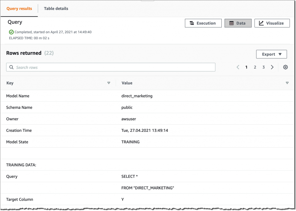
As anticipated, the mannequin is at present within the TRAINING state.
Once I created this mannequin, I chosen all of the columns within the desk as enter parameters. I’m wondering what occurs if I create a mannequin that makes use of fewer enter parameters? I’m within the cloud and I’m not slowed down by restricted assets, so I create one other mannequin utilizing a subset of the columns within the desk:
CREATE MODEL simple_direct_marketing
FROM (
        SELECT age, job, marital, schooling, housing, contact, month, day_of_week, y
 	  FROM direct_marketing
)
TARGET y
FUNCTION predict_simple_direct_marketing
IAM_ROLE 'arn:aws:iam::123412341234:position/RedshiftML'
SETTINGS (
  S3_BUCKET 'my-bucket'
);
After a while, my first mannequin is prepared, and I get this output from SHOW MODEL. The precise output within the console is in a number of pages, I merged the outcomes right here to make it simpler to observe:

From the output, I see that the mannequin has been appropriately acknowledged as BinaryClassification, and F1 has been chosen as the target. The F1 rating is a metrics that considers each precision and recall. It returns a price between 1 (good precision and recall) and zero (lowest attainable rating). The ultimate rating for the mannequin (validation:f1) is zero.79. On this desk I additionally discover the title of the SQL operate (predict_direct_marketing) that has been created for the mannequin, its parameters and their varieties, and an estimation of the coaching prices.
When the second mannequin is prepared, I examine the F1 scores. The F1 rating of the second mannequin is decrease (zero.66) than the primary one. Nevertheless, with fewer parameters the SQL operate is simpler to use to new information. As is commonly the case with machine studying, I’ve to seek out the correct steadiness between complexity and value.
Utilizing Redshift ML to Make Predictions
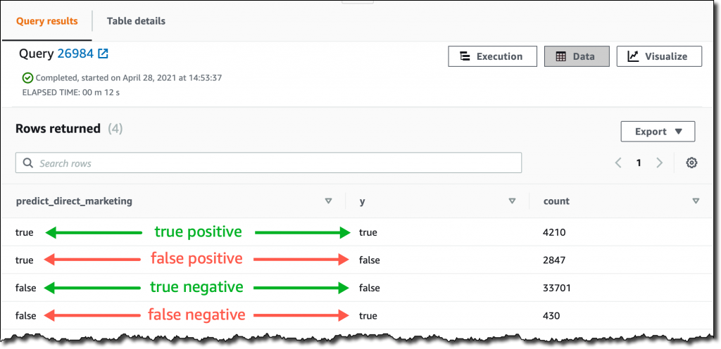
Now that the 2 fashions are prepared, I could make predictions utilizing SQL features. Utilizing the primary mannequin, I test what number of false positives (fallacious constructive predictions) and false negatives (fallacious damaging predictions) I get when making use of the mannequin on the identical information used for coaching:
SELECT predict_direct_marketing, y, COUNT
  FROM (SELECT predict_direct_marketing(
                   age, job, marital, schooling, credit_default, housing,
                   mortgage, contact, month, day_of_week, period, marketing campaign,
                   pdays, earlier, poutcome, emp_var_rate, cons_price_idx,
                   cons_conf_idx, euribor3m, nr_employed), y
          FROM direct_marketing)
 GROUP BY predict_direct_marketing, y;
The results of the question reveals that the mannequin is best at predicting damaging somewhat than constructive outcomes. In actual fact, even when the variety of true negatives is far greater than true positives, there are rather more false positives than false negatives. I added some feedback in inexperienced and pink to the next screenshot to make clear the which means of the outcomes.
Utilizing the second mannequin, I see what number of clients is likely to be enthusiastic about a advertising marketing campaign. Ideally, I ought to run this question on new buyer information, not the identical information I used for coaching.
SELECT COUNT
  FROM direct_marketing
 WHERE predict_simple_direct_marketing(
           age, job, marital, schooling, housing,
           contact, month, day_of_week) = true;
Wow, wanting on the outcomes, there are greater than 7,000 prospects!

Availability and Pricing
Redshift ML is accessible as we speak within the following AWS Areas: US East (Ohio), US East (N Virginia), US West (Oregon), US West (San Francisco), Canada (Central), Europe (Frankfurt), Europe (Eire), Europe (Paris), Europe (Stockholm), Asia Pacific (Hong Kong) Asia Pacific (Tokyo), Asia Pacific (Singapore), Asia Pacific (Sydney), and South America (São Paulo). For extra data, see the AWS Regional Providers listing.
With Redshift ML, you pay just for what you employ. When coaching a brand new mannequin, you pay for the Amazon SageMaker Autopilot and S3 assets utilized by Redshift ML. When making predictions, there isn’t a extra price for fashions imported into your Amazon Redshift cluster, as within the instance I used on this publish.
Redshift ML additionally permits you to use present Amazon SageMaker endpoints for inference. In that case, the standard SageMaker pricing for real-time inference applies. Right here yow will discover just a few tips about learn how to management your prices with Redshift ML.
To study extra, you’ll be able to see this weblog publish from when Redshift ML was introduced in preview and the documentation.
Begin getting higher insights out of your information with Redshift ML.
— Danilo
[ad_2]
Source link